Hướng Dẫn Vẽ Đồ Thị 3D trong MuPAD Của MatLab

Hướng Dẫn Vẽ Đồ Thị 3D trong MuPAD Của MatLab

plot::Function3d – 3D function graphs

plot::Function3d creates the 3D graph of a function in 2 variables.

Calls:

plot::Function3d(f, Options)

plot::Function3d(f, x = .. , y = .. , <a = a_min .. a_max>, Options)

Parameters:

f:	the function: an arithmetical expression or a piecewise object in the independent variables , and the animation parameter a. Alternatively, a MuPAD procedure that accepts 2 input parameter , or 3 input parameters , , and returns a numerical value when the input parameters are numerical.   f is equivalent to the attribute Function.
x:	the first independent variable: an identifier or an indexed identifier.   x is equivalent to the attribute XName.
.. :	the plot range in direction: , must be numerical real values or expressions of the animation parameter . If not specified, the default range x = -5 .. 5 is used.   .. is equivalent to the attributes XRange, XMin, XMax.
y:	the second independent variable: an identifier or an indexed identifier.   y is equivalent to the attribute YName.
.. :	the plot range in direction: , must be numerical real values or expressions of the animation parameter . If not specified, the default range y = -5 .. 5 is used.   .. is equivalent to the attributes YRange, YMin, YMax.

See Also:

plot, plot::copy, plot::Function2d, plot::Surface, plotfunc2d, plotfunc3d

Details:

·                     The expression f(x, y) is evaluated at finitely many points , in the plot range. There may be singularities. Although a heuristics is used to find a reasonable range when singularities are present, it is highly recommended to specify a range via ViewingBoxZRange = with suitable numerical real values , . Cf. example 2.

·                     Animations are triggered by specifying a range for a parameter a that is different from the indedependent variables x, y. Thus, in animations, the -range , the -range as well as the animation range must be specified. Cf. example 3.

·                     The function f is evaluated on a regular equidistant mesh of sample points determined by the attributes XMesh and YMesh (or the shorthand-notation for both, Mesh). By default, the attribute AdaptiveMesh = 0 is set, i.e., no adaptive refinement of the equidistant mesh is used.

If the standard mesh does not suffice to produce a sufficiently detailed plot, one may either increase the value of XMesh and YMesh or set AdaptiveMesh = n with some (small) positive integer n. This may result in up to times as many triangles as used with AdaptiveMesh = 0, potentially more when f has non-isolated singularities. Cf. example 4.

·                     The “coordinate lines” (“parameter lines”) are curves on the function graph.

The phrase “XLines” refers to the curves with the parameter running from to , while is some fixed value from the interval .

The phrase “YLines” refers to the curves with the parameter running from ymin to ymax, while is some fixed value from the interval .

By default, the parameter lines are visible. They may be “switched off” by specifying XLinesVisible = FALSE and YLinesVisible = FALSE, respectively.

·                     The coordinate lines controlled by XLinesVisible = TRUE/FALSE and YLinesVisible = TRUE/FALSE indicate the equidistant regular mesh set via the Mesh attributes. If the mesh is refined by the Submesh attributes or by the adaptive mechanism controlled by AdaptiveMesh = n, no additional parameter lines are drawn.

As far as the numerical approximation of the function graph is concerned, the settings

,

and

, Submesh = [0, 0]

are equivalent. However, in the first setting, nx parameter lines are visible in the direction, while in the latter setting parameter lines are visible. Cf. example 5.

Attributes for plot::Function3d

AdaptiveMesh = 0	adaptive sampling
AffectViewingBox = TRUE	influence of objects on the ViewingBox of a scene
Color = RGB::Red	the main color
FillColor = RGB::Red	color of areas and surfaces
FillColor2 = RGB::CornflowerBlue	second color of areas and surfaces for color blends
FillColorDirection = [0, 0, 1]	the direction of color transitions on surfaces
FillColorDirectionX = 0	x-component of the direction of color transitions on surfaces
FillColorDirectionY = 0	y-component of the direction of color transitions on surfaces
FillColorDirectionZ = 1	z-component of the direction of color transitions on surfaces
FillColorFunction	functional area/surface coloring
FillColorType = Dichromatic	surface filling types
Filled = TRUE	filled or transparent areas and surfaces
Frames = 50	the number of frames in an animation
Function	function expression or procedure
Legend	makes a legend entry
LegendEntry = TRUE	add this object to the legend?
LegendText	short explanatory text for legend
LineColor = RGB::Black.[0.25]	color of lines
LineColor2 = RGB::DeepPink	color of lines
LineColorDirection = [0, 0, 1]	the direction of color transitions on lines
LineColorDirectionX = 0	x-component of the direction of color transitions on lines
LineColorDirectionY = 0	y-component of the direction of color transitions on lines
LineColorDirectionZ = 1	z-component of the direction of color transitions on lines
LineColorFunction	functional line coloring
LineColorType = Flat	line coloring types
LineStyle = Solid	solid, dashed or dotted lines?
LinesVisible = TRUE	visibility of lines
LineWidth = 0.35	width of lines
Mesh = [25, 25]	number of sample points
MeshVisible = FALSE	visibility of irregular mesh lines in 3D
Name	the name of a plot object (for browser and legend)
ParameterBegin	initial value of the animation parameter
ParameterEnd	end value of the animation parameter
ParameterName	name of the animation parameter
ParameterRange	range of the animation parameter
PointSize = 1.5	the size of points
PointStyle = FilledCircles	the presentation style of points
PointsVisible = FALSE	visibility of mesh points
Shading = Smooth	smooth color blend of surfaces
Submesh = [0, 0]	density of submesh (additional sample points)
TimeBegin = 0.0	start time of the animation
TimeEnd = 10.0	end time of the animation
TimeRange = 0.0 .. 10.0	the real time span of an animation
Title	object title
TitleAlignment = Center	horizontal alignment of titles w.r.t. their coordinates
TitleFont = ["sans-serif", 11]	font of object titles
TitlePosition	position of object titles
TitlePositionX	position of object titles, x component
TitlePositionY	position of object titles, y component
TitlePositionZ	position of object titles, z component
Visible = TRUE	visibility
VisibleAfter	object visible after this time value
VisibleAfterEnd = TRUE	object visible after its animation time ended?
VisibleBefore	object visible until this time value
VisibleBeforeBegin = TRUE	object visible before its animation time starts?
VisibleFromTo	object visible during this time range
XLinesVisible = TRUE	visibility of parameter lines (x lines)
XMax = 5	final value of parameter “x”
XMesh = 25	number of sample points for parameter “x”
XMin = -5	initial value of parameter “x”
XName	name of parameter “x”
XRange = -5 .. 5	range of parameter “x”
XSubmesh = 0	density of additional sample points for parameter “x”
YLinesVisible = TRUE	visibility of parameter lines (y lines)
YMax = 5	final value of parameter “y”
YMesh = 25	number of sample points for parameter “y”
YMin = -5	initial value of parameter “y”
YName	name of parameter “y”
YRange = -5 .. 5	range of parameter “y”
YSubmesh = 0	density of additional sample points for parameter “y”
ZContours	contour lines at constant z values

Example 1

The following call returns an object representing the graph of the function over the region , : g := plot::Function3d(sin(x^2 + y^2), x = -2..2, y = -2..2) Call plot to plot the graph: plot(g) Functions can also be specified by piecewise objects or procedures: f := piecewise([x < y, 0], [x >= y, (x - y)^2]): plot(plot::Function3d(f, x = -2 .. 4, y = -1 .. 3)) f := proc(x, y) begin   if x + y^2 + 2*y < 0 then      0   else      x + y^2 + 2*y   end_if: end_proc: plot(plot::Function3d(f, x = -3 .. 2, y = -2 .. 2)) delete g, f

Example 2

We plot a function with singularities: f := plot::Function3d(x/y + y/x, x = -1 .. 1, y = - 1 .. 1): plot(f) We specify an explicit viewing range for the direction: plot(f, ViewingBoxZRange = -20 .. 20) delete f

Example 3

We generate an animation of a parametrized function: plot(plot::Function3d(sin((x - a)^2 + y^2),                       x = -2 .. 2, y = -2 .. 2, a = 0 .. 5))

Example 4

The standard mesh for the numerical evaluation of a function graph does not suffice to generate a satisfying graphics in the following case: plot(plot::Function3d(besselJ(0, sqrt(x^2 + y^2)),                       x = -20 .. 20, y = -20 .. 20)) We increase the number of mesh points. Here, we use XSubmesh and YSubmesh to place 2 additional points in each direction between each pair of neighboring points of the default mesh. This increases the runtime by a factor of : plot(plot::Function3d(besselJ(0, sqrt(x^2 + y^2)),                       x = -20 .. 20, y = -20 .. 20,                       Submesh = [2, 2])) Alternatively, we enable adaptive sampling by setting the value of AdaptiveMesh to some positive value: plot(plot::Function3d(besselJ(0, sqrt(x^2 + y^2)),                       x = -20 .. 20, y = -20 .. 20,                       AdaptiveMesh = 2))

Example 5

By default, the parameter lines of a function graph are “switched on”: plot(plot::Function3d(x^2 + y^2, x = 0 .. 1, y = 0 .. 1)) The parameter lines are “switched off” by setting XLinesVisible, YLinesVisible: plot(plot::Function3d(x^2 + y^2, x = 0 .. 1, y = 0 .. 1,                       XLinesVisible = FALSE,                       YLinesVisible = FALSE)) The number of parameter lines are determined by the Mesh attributes: plot(plot::Function3d(x^2 + y^2, x = 0 .. 1, y = 0 .. 1,                       Mesh = [5, 12])) When the mesh is refined via the Submesh attributes, the numerical approximation of the surface becomes smoother. However, the number of parameter lines is not increased: plot(plot::Function3d(x^2 + y^2, x = 0 .. 1, y = 0 .. 1,                       Mesh = [5, 12],                       XSubmesh = 1, YSubmesh = 2))

Example 6

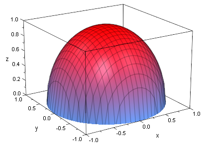
Functions need not be defined over the whole parameter range: plot(plot::Function3d(sqrt(1-x^2-y^2), x=-1..1, y=-1..1)) plot(plot::Function3d(sqrt(sin(x)+cos(y)))) This makes for an easy way of plotting a function over a non-rectangular area: chi := piecewise([x^2 < abs(y), 1]) plot(plot::Function3d(chi*sin(x+cos(y))),      CameraDirection=[-1,0,0.5])  Tải File Hướng Dẫn